OSFP AI Networking: Architecting GPU Clusters for Distributed Training

March 31, 2026

FiberMall

One-stop supplier of professional optical communication products

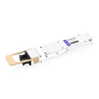
The optical transceiver market for AI infrastructure is projected to reach $4.5 billion by 2025, with OSFP modules driving the majority of this growth. The current AI training clusters need network bandwidth that exceeds the capabilities that existed five years earlier. The process of training a large language model requires 400 terabytes of network traffic per hour because 25,000 GPUs need to use all-reduce operations, which consume 90 percent of their available bandwidth.

The existing data center networks lack the capacity to handle these particular workloads. The three-tier architecture system creates excessive delays because it suffers from multiple oversubscription points. Standard Ethernet without RDMA capabilities leaves GPUs idle, waiting for gradient synchronization. The network strength defines the operational efficiency of expensive GPU clusters because it decides whether the system achieves 90 percent usage or incurs million-dollar losses.

The guide presents an entire system that shows how to build AI training networks with OSFP technology. The training program will explain to you the networking infrastructure requirements for AI training, the OSFP technology which supports large-scale fabric development, the network designs that major AI systems use, and how to create your own GPU cluster network.

For comprehensive OSFP technology fundamentals, see our complete guide to OSFP transceivers.

Table of Contents

Why AI Training Requires Specialized Networking

The All-Reduce Bottleneck

The distributed AI training process uses all-reduce operations to achieve gradient synchronization between all GPUs present in the cluster. Every training iteration requires each GPU to compute its data gradients before sharing these gradients with all other GPUs for model parameter updates.

The all-reduce pattern functions as the primary network traffic generator. According to industry tests, all-reduce operations use 89% of network bandwidth during the training of large models. The remaining 11% covers checkpointing, logging, and management traffic.

Consider a concrete example: training a 70 billion parameter model across 512 GPUs with the Adam optimizer uses 32-bit floating point precision. Each GPU maintains:

Model parameters: 140 GB (70B × 2 bytes)
Optimizer states (momentum and variance): ~280 GB
Gradients: 140 GB

Every training iteration requires synchronizing 140 GB of gradient data across all 512 GPUs. With synchronous training requiring updates every 1-2 seconds, the network must sustain:

140 GB/s aggregate bandwidth for gradient all-reduce
Bi-directional traffic (each GPU sends and receives gradients)
Bursty patterns (all GPUs communicate simultaneously during all-reduce)

Traditional networks collapse under this load. Training stalls because oversubscribed architectures create network congestion. The absence of RDMA causes CPUs to handle data transfers which results in delays that prevent GPUs from operating. The network waits for millions of dollars in GPU capacity which results in wasted time.

Bandwidth Requirements by Scale

Network requirements scale proportionally with model size and GPU count. The following table shows approximate requirements for different training scales:

Model Size	GPU Count	Aggregate Bandwidth	Checkpoint Size	Daily Traffic
7B	64	20 GB/s	14 GB	~2 PB
70B	512	140 GB/s	140 GB	~12 PB
175B	1,024	350 GB/s	350 GB	~30 PB
1T	8,192	2 TB/s	2 TB	~200 PB
GPT-4 scale	25,000	8.5 TB/s	5 TB+	~400 TB/hr

These figures assume FP16/BF16 training with synchronous SGD or Adam optimizers. Quantization to 8-bit precision reduces bandwidth requirements by 50%, which is why many large-scale deployments use mixed-precision training.

Checkpointing adds additional storage bandwidth requirements. A 175B parameter model checkpoint includes:

Model weights: 350 GB (FP16)
Optimizer states: ~700 GB (Adam)
Total: ~1.05 TB per checkpoint

At a checkpoint frequency of every 1,000 iterations with 2-second iteration time, the storage system must write 1.05 TB every 33 minutes, requiring 525 MB/s sustained write bandwidth per checkpoint stream. Parallel checkpoints from multiple nodes can saturate storage networks.

Latency vs Throughput

AI training networks have different requirements than traditional applications:

Throughput dominates: The training process requires continuous high bandwidth because it needs to transfer large amounts of gradient data. The difference between a training iteration that takes 1.5 seconds and one that takes 1.4 seconds results in two completed training iterations who take their time.

Latency still matters: Microsecond-scale latency affects GPU utilization. When gradients arrive late, GPUs sit idle, reducing effective utilization. The usage requirement for this system remains less strict than the requirements for inference and HPC simulation programs.

InfiniBand NDR: The technology achieves sub-microsecond latency through its 600ns port-to-port latency which enables precise synchronization needed for advanced models that require every millisecond of training time.

RoCEv2: The technology delivers 2 microsecond latency which most training workloads can handle while it delivers major cost benefits compared to InfiniBand.

The key metric is GPU utilization percentage. Well-designed networks achieve 85-95% GPU utilization during training. Poorly designed networks with bottlenecks may see utilization drop to 50-60%, effectively doubling training time and cost.

OSFP: The Form Factor for AI Infrastructure

Why OSFP Dominates AI Networks

OSFP has become the principal optical standard for AI infrastructure which has replaced QSFP-DD in all new high-performance installations. The following technical elements determine the preferential choice:

Thermal Headroom: AI workloads will push optical modules to their maximum powered operation. The power consumption of 800G OSFP modules ranges from 15 to 25 watts while their coherent models exceed 25 watts. The OSFP integrated heat sink design offers 30 percent more surface area compared to QSFP-DD which enables safe operation at these power levels. The larger form factor accommodates more substantial thermal management, critical for maintaining signal integrity at 112G PAM4.

Native 800G Support: OSFP was designed for 800G from inception, with eight electrical lanes each running 112G PAM4. The 800G connection of QSFP-DD requires higher lane rates which operate at 200G per lane in QSFP-DD800 but this increases both power usage and signal integrity problems.

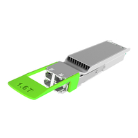
1.6T Migration Path: The OSFP-XD (eXtended Density) variant extends the form factor for 1.6T operation while maintaining the same management interface and cage compatibility. Hyperscale contracts specify OSFP-XD in 92% of 1.6T deployments.

Twin-Port Design: Many 800G OSFP modules implement twin-port architecture, internally presenting as two 400G ports. The system enables users to connect directly to dual-port ConnectX-7 NICs without needing additional breakout cables which improves both cabling efficiency and insertion loss performance.

OSFP InfiniBand NDR

InfiniBand NDR (Next Data Rate) provides 400G per-port transport capability and serves as the foundational link for high-performance AI fabrics. The technology stack includes:

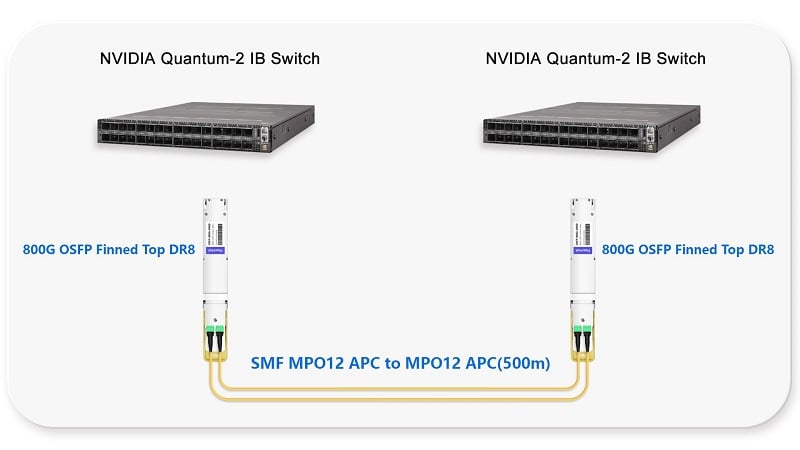
Physical Layer: Each 400G port uses 4 × 100G PAM4 lanes. It employs twin-port 800G OSFP modules (a single OSFP cage supports 2 × 400G NDR). The OSFP module handles electrical-to-optical conversion with its transmitters operating at 1310nm for DR8 variants.

Protocol Stack: InfiniBand provides hardware-managed reliable transport with native RDMA support. The network interface card (NIC) implements transport protocols in hardware which enables zero-copy data transfers between GPU memory and the network.

Latency Performance: End-to-end latency reaches 600 nanoseconds through the connection from one port to another between leaf and spine links. This technology allows all-reduce operations to finish within microseconds instead of taking multiple milliseconds.

Congestion Management: InfiniBand uses credit-based flow control together with adaptive routing technology to stop all GPUs from creating congestion hotspots during all-reduce storms.

NVIDIA Quantum-2 switches use InfiniBand NDR technology through 64× 800G OSFP ports which deliver 51.2 Tbps switching capacity within a single chassis. This density makes it possible to create clusters containing more than 8,000 GPUs using only two switching tiers.

OSFP RoCEv2 Implementation

RoCEv2 (RDMA over Converged Ethernet v2) provides an Ethernet-based alternative to InfiniBand for organizations seeking lower costs or standard Ethernet management tools.

Requirements for Lossless Operation:

PFC (Priority Flow Control): IEEE 802.1Qbb pause frames prevent buffer overflow during congestion
ECN (Explicit Congestion Notification): IEEE 802.1Qau marks packets before congestion builds, enabling senders to reduce rates
DCQCN (Data Center Quantized Congestion Notification): Combines ECN with rate limiting for TCP-friendly congestion control

Performance Characteristics:

Latency: ~2 microseconds (3× InfiniBand but still excellent)
Throughput: Equivalent to InfiniBand for most workloads
Cost: 30-40% lower than equivalent InfiniBand infrastructure
Scale: Proven at 8,000+ GPU scale (Meta’s deployment)

When to Choose RoCEv2:

Cost-sensitive deployments
Existing Ethernet management expertise
Workloads tolerant of slightly higher latency
Infrastructure shared with non-AI traffic

Meta’s SIGCOMM 2024 paper demonstrates RoCEv2 operating at hyperscale for LLM training, validating Ethernet as a viable alternative to InfiniBand for most AI workloads.

AI Cluster Architecture with OSFP

Spine-Leaf (Fat-Tree) Topology

Modern AI clusters universally adopt spine-leaf (also called fat-tree or Clos) topology for their backend networks. This architecture provides:

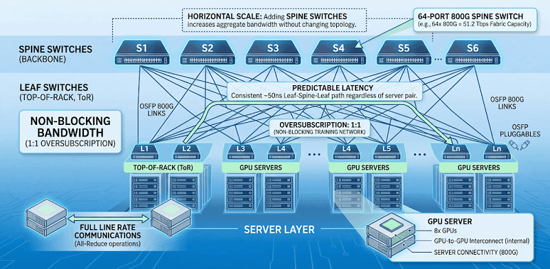
Non-Blocking Bandwidth: With 1:1 oversubscription between leaf and spine tiers, every server can communicate with every other server at full line rate simultaneously. This is essential for all-reduce operations where all GPUs communicate with all others.

Predictable Latency: Every server-to-server path traverses exactly two switches (leaf → spine → leaf), providing consistent ~50 nanosecond leaf-spine latency regardless of which servers communicate.

Horizontal Scale: Adding spine switches increases aggregate bandwidth without changing the fundamental topology. A 64-port spine switch adds 64× 800G = 51.2 Tbps of fabric capacity.

Two-Tier Design:

Leaf switches: Top-of-rack, connect directly to GPU servers
Spine switches: Backbone, connect all leaf switches in full mesh
Oversubscription: 1:1 for training networks (no oversubscription)

Example configuration for 2,048 GPUs:

32 leaf switches (64 ports each, 400G down to servers, 800G up)
32 spine switches (64 ports each, all 800G)
Each leaf connects to each spine (full mesh)
Total fabric capacity: 32 × 51.2 Tbps = 1.64 Pbps

Rail-Optimized Design

NVIDIA’s DGX SuperPOD architecture introduced rail-optimized networking, which optimizes physical connectivity for tensor parallelism patterns.

The Concept: In multi-GPU servers, GPUs are arranged in “rails” corresponding to their position in the server chassis. Rail-optimized networking connects GPUs in the same rail position across all servers to the same leaf switch.

Example: DGX H100 with 8 GPUs:

GPU 0 from all servers → Leaf Switch 0
GPU 1 from all servers → Leaf Switch 1
…
GPU 7 from all servers → Leaf Switch 7

Benefits:

Minimizes switch hops for tensor parallelism (intra-rail communication stays on one leaf)
Reduces spine traffic for common communication patterns
Improves all-reduce performance for distributed training frameworks

Implementation with OSFP:
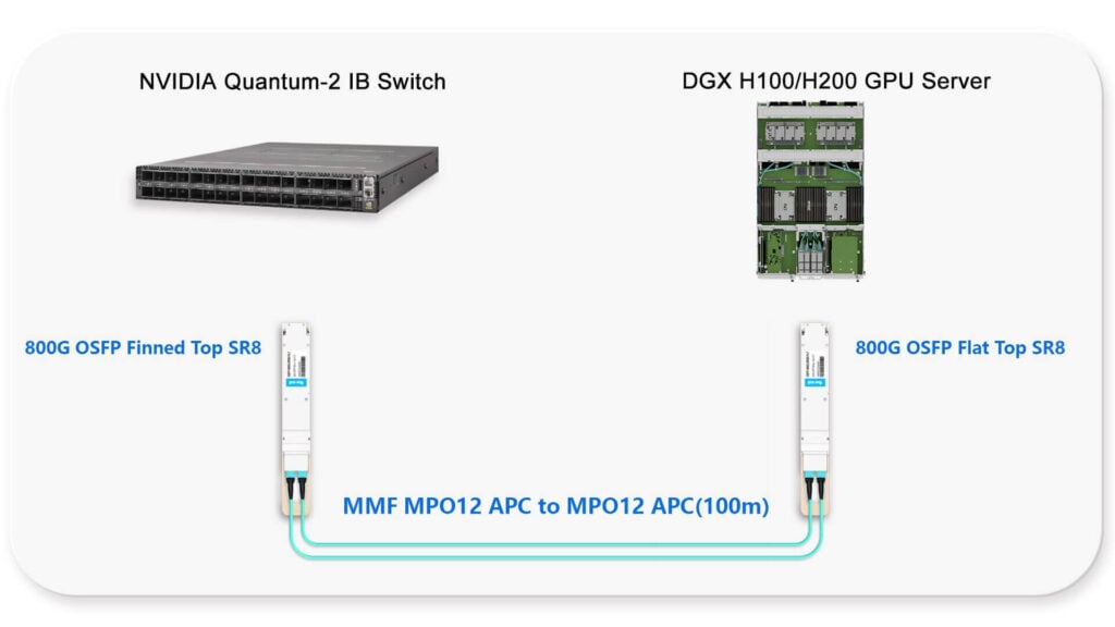
Each DGX H100 has 8× 400G ConnectX-7 NICs. Using 800G OSFP modules with twin-port breakout:

800G OSFP → 2× 400G connections
4× 800G OSFP ports serve 8× 400G NICs
MPO-16 cables carry 8 lanes for 800G, breaking out to MPO-8 for 400G

Scale Calculations

51.2T Fabric (800G OSFP):

64-port 800G spine switches
Each spine: 64 × 800G = 51.2 Tbps capacity
32 spines provide 1.64 Pbps total fabric
Supports 8,192 GPUs (1,024 servers × 8 GPUs)

Multi-POD Architecture:
For clusters exceeding single-fabric scale, Meta’s architecture adds a third tier:

RTSW (Rack Training Switch): Leaf tier
CTSW (Cluster Training Switch): Spine tier within AI Zone
ATSW (Aggregator Training Switch): Connects multiple AI Zones

The ATSW tier typically operates with 3:1 or 4:1 oversubscription since cross-zone traffic is less frequent than intra-zone communication. Topology-aware job scheduling places related jobs within the same zone to minimize cross-zone traffic.

Real-World Example: NVIDIA DGX H100 SuperPOD

A DGX H100 SuperPOD implements rail-optimized spine-leaf architecture with specific components:

Server Configuration:

8× NVIDIA H100 GPUs per server
8× ConnectX-7 400G NICs (one per GPU)
2× additional NICs for storage/management
4× 800G OSFP ports (twin-port serving 8× 400G)

Network Configuration:

32 leaf switches (rail-optimized)
16 spine switches
All-OSFP infrastructure (800G leaf-spine, 400G to servers)
InfiniBand NDR or RoCEv2 protocol

Cabling:

Intra-rack: DAC for <3m, AOC for 3-30m
Leaf-spine: OSFP DR8 single-mode fiber
Total: ~576 OSFP modules per 32-node pod

This architecture delivers 90%+ GPU utilization for large-scale distributed training.

The Fiber Explosion: Cabling AI Clusters

Per-Server Fiber Requirements

AI servers require staggering amounts of fiber connectivity compared to traditional servers. A DGX H100 exemplifies this:

AI Network:

8× 400G ConnectX-7 NICs
4× 800G OSFP modules (twin-port breakout)
8× MPO-16 connectors (one per 800G module)
128 fibers (8 modules × 16 fibers)

Storage/Compute Network:

2× 200G NICs (minimum)
2× MPO-12 or MPO-8 connectors
16-24 fibers

Total per Server: 10 OSFP ports, 144-152 fibers

This is 10-20× the fiber count of a standard application server with dual 25G connections.

Per-Rack Calculations

A typical AI rack contains 4 DGX H100 servers:

AI Network:

4 servers × 8 AI NICs = 32× 400G connections
Or 16× 800G OSFP ports
256 fibers for AI traffic

Storage Network:

4 servers × 2 storage NICs = 8× 200G connections
64 fibers for storage

Total per Rack: 320 fibers (before redundancy or management)

For a 42U rack, this leaves minimal space for patch panels and cable management. Specialized high-density fiber solutions become mandatory.

Cluster-Scale Numbers

A 4,000 GPU cluster (500 DGX H100 servers) requires:

OSFP Modules:

2,000× 800G modules (leaf-spine + server connections)
Plus spares: 200-300 modules

Fiber Connections:

100,352 MPO connections (500 servers × 200 fibers average)
Plus patch panel interconnections

Cable Length:

Average 50m per fiber pair
5,000+ km of fiber total

Structured cabling is essential. Point-to-point jumper cables create an unmaintainable mess at this scale. Pre-terminated trunk cables with MPO connectors reduce installation time and improve reliability.

Fiber Types by Application

Type	Distance	Use Case	Connector
SR8	100m	Intra-rack, adjacent racks	MPO-16 (MMF)
DR8	500m	Leaf-spine within building	MPO-16 (SMF)
FR8	2km	Multi-building campus	MPO-16 (SMF)
LR8	10km	DCI, metro	MPO-16 (SMF)
AOC	30m	Intra-rack	OSFP integrated
DAC	3m	Within same rack	OSFP integrated

Single-mode fiber dominates AI deployments due to lower loss and future-proofing for higher speeds. Multimode remains viable only for highest-density, shortest-reach applications where cost is the primary constraint.

Network Protocols: InfiniBand vs RoCE

InfiniBand NDR

InfiniBand remains the premium choice for highest-performance AI training:

Advantages:

Lowest latency: <1μs end-to-end, 600ns switch-to-switch
Hardware RDMA: Zero-copy transfers, CPU bypass
Native congestion control: Credit-based flow control prevents drops
Proven at scale: 32,000+ GPU deployments operational
Ecosystem: Optimized collective libraries (NCCL, RCCL)

Components:

NVIDIA Quantum-2 switches (64× 800G OSFP)
ConnectX-7/8 NICs (400G/800G)
InfiniBand NDR cables (passive copper or active optical)

Cost: Premium pricing, approximately 30-40% higher than equivalent Ethernet infrastructure.

RoCEv2 over Ethernet

RoCEv2 has emerged as a viable, lower-cost alternative:

Advantages:

Standard Ethernet: Use existing switches, management tools
Lower cost: 30-40% savings vs InfiniBand
Proven at hyperscale: Meta’s 8,000+ GPU deployment
Flexibility: Easier to share infrastructure with non-AI workloads

Requirements:

Lossless Ethernet: PFC + ECN mandatory
Deep buffer switches: Handle incast during all-reduce
RDMA-capable NICs: ConnectX-7 or equivalent

Configuration:

Enable PFC on specific priority class (typically 3)
Configure ECN thresholds
Implement DCQCN for congestion control
Use DCBX for automatic configuration exchange

Performance:

Latency: ~2μs (acceptable for most training)
Throughput: Equivalent to InfiniBand for large transfers
GPU utilization: 85-90% achievable with proper tuning

Selection Decision Matrix

Factor	InfiniBand NDR	RoCEv2
Latency	<1μs	~2μs
Cost	Premium (base + 40%)	Standard
Management	Proprietary (UFM)	Standard Ethernet
Scale	32,000+ GPUs proven	8,000+ GPUs proven
Ecosystem	NVIDIA-optimized	Broader vendor support
Best For	Frontier LLMs, HPC	Most AI training workloads

Decision Guidance:

Choose InfiniBand for maximum performance, NVIDIA-centric environments, or when every microsecond counts
Choose RoCEv2 for cost optimization, multi-vendor environments, or when leveraging existing Ethernet expertise

Both protocols benefit from OSFP’s high-density, high-bandwidth capabilities.

Cost Analysis: AI Networking Economics

Network as % of AI Cluster

Networking represents a significant but often underestimated portion of AI infrastructure costs:

Typical Breakdown:

GPUs: 60-70% of cluster cost
Servers (CPU, memory, storage): 15-20%
Networking (switches, NICs, optics, cabling): 8-12%
Facilities (power, cooling, rack): 5-10%

For a 1,024 GPU cluster:

Total investment: ~$30-40M
Networking: ~$2.5-4M (8-12%)
- Switches: $1.5M
- NICs: $0.8M
- Optics/cables: $0.5M

While networking is a smaller percentage than compute, optimization matters. A 20% reduction in network costs saves $500K-800K on a large cluster.

Per-Port Costs

InfiniBand NDR (800G):

Switch port: ~$1,500-2,000
OSFP module: ~$800-1,200
Cable (30m AOC): ~$300
Total per link: ~$2,600-3,500

RoCEv2 (800G):

Switch port: ~$1,000-1,500
OSFP module: ~$800-1,200
Cable (30m AOC): ~$300
Total per link: ~$2,100-3,000

Per-GPU networking cost: ~$3,000-5,000 depending on topology and protocol.

Optimization Strategies

Use DAC for short distances:

DAC cables cost 50-70% less than AOC
Use for all intra-rack connections (<3m)
Significant savings: 30-40% of cables can be DAC in typical deployments

Right-size oversubscription:

Training networks need 1:1 (non-blocking)
Storage networks can tolerate 3:1 or 4:1
Management networks: 10:1 acceptable

Optimize fiber type:

SR8 (multimode) costs 30-40% less than DR8 (single-mode)
Use SR8 for intra-rack and adjacent rack connections
Reserve DR8 for leaf-spine and longer runs

Consider LPO for short reach:

Linear Pluggable Optics reduce power and cost
30-50% savings on optics for <2km reaches
Limited availability but growing adoption

The Underutilization Penalty:

If a $40M cluster runs at 60% GPU utilization instead of 90% due to network bottlenecks:

Effective capacity: 614 GPUs vs 922 GPUs
Wasted investment: $13.3M equivalent
Annual cloud cost equivalent: $400K+ in wasted on-premise investment

Spending an extra $500K on network optimization to achieve 90% vs 60% utilization pays for itself immediately.

Future of AI Networking

1.6T OSFP-XD

The transition to 1.6T is underway, with OSFP-XD as the dominant form factor:

Timeline:

2025: Early production for hyperscalers
2026: Volume production (30M+ units projected)
2027: Mainstream adoption

Technical Specifications:

12 lanes × 133 Gbps = 1.6 Tbps
Same physical width as OSFP, slightly taller
Backward compatible with OSFP cages (mechanical)
Power: 25-30W per module

Impact on AI Clusters:

Doubles fabric capacity with same switch port count
64-port 1.6T switch = 102.4 Tbps fabric
Enables 16,000+ GPU clusters with two-tier topology

Hyperscale Adoption: 92% of 1.6T contracts specify OSFP-XD over alternatives.

Linear Pluggable Optics (LPO)

LPO eliminates the DSP (Digital Signal Processor) from optical modules, reducing power and latency:

Benefits:

Power reduction: 30-50% (10-14W vs 18-25W for 800G)
Latency: ~15ns reduction
Cost: 20-30% lower module cost

Trade-offs:

Shorter reach: <2km typically
Stricter host requirements: Switch must provide signal conditioning
Limited management: Reduced telemetry capabilities

Adoption Forecast: 40% of short-reach 800G links in AI data centers by late 2025.

NVIDIA Spectrum-X and Meta AI networks already deploy LPO for intra-data center connectivity.

Co-Packaged Optics (CPO)

CPO represents the next major architecture shift:

Concept: Integrate optical engines directly with switch ASICs, eliminating pluggable modules.

Benefits:

Power reduction: 40-50% vs pluggable optics
Bandwidth density: 10× increase
Latency: Eliminates PCB trace losses

Timeline:

2025-2026: Field trials with 51.2T switches
2028-2030: Volume deployment

Challenges:

Serviceability: Cannot replace individual optics
Thermal: Concentrated heat from integrated optics
Ecosystem: Limited vendor support initially

Jensen Huang’s Perspective: Scaling to 1 million GPUs with traditional pluggables would consume 180MW just for optics—described as “unsustainable.” CPO is essential for future hyperscale AI.

For organizations building infrastructure today, design for pluggable optics but plan for CPO migration in the 2028+ timeframe.

Troubleshooting AI Network Issues

Common Problems and Solutions

Symptom	Likely Cause	Solution
Low GPU utilization (<70%)	Network bottleneck in all-reduce	Check effective bandwidth; verify no congestion
Training slowdown after N iterations	Congestion building up	Tune ECN thresholds; check for hot spots
Link flapping during peak load	Thermal issues	Verify cooling; check DOM temperatures
Inconsistent iteration times	Job placement across zones	Use topology-aware scheduling
High latency on some flows	ECMP imbalance	Verify flow distribution; consider adaptive routing
GPU synchronization timeouts	Packet loss	Enable and verify PFC; check for drops

Key Metrics to Monitor

Network Metrics:

All-reduce completion time (target: <100ms for large clusters)
Effective bandwidth vs theoretical maximum
Per-port utilization during all-reduce
Buffer occupancy (should never reach 100%)

GPU Metrics:

GPU utilization percentage (target: 85-95%)
Time waiting for gradients (should be <10% of iteration)
PCIe bandwidth utilization
Memory bandwidth utilization

System Metrics:

Job completion time vs ideal
Checkpoint write bandwidth
Recovery time after failure

Diagnostic Commands

InfiniBand:

# Check link status

ibstatus

# Verify link speed

ibstat

# Check for errors

perfquery

# Monitor congestion

ibtracert

RoCEv2:

# Check PFC configuration

lldptool get-tlv -i eth0 -c pfc

# Monitor ECN counters

cat /sys/class/net/eth0/ecn/stats

# Check RDMA connection status

rdma link show

# Verify GID configuration

rdma dev show

Frequently Asked Questions

How many GPUs can 800G OSFP support?

The 64-port 800G spine switch delivers a total fabric capacity of 51.2 Tbps. The system enables 8,192 GPUs to operate through two-tier spine-leaf architecture with servers that use eight GPUs each. The three-tier system with aggregator switches allows organizations to develop their clusters which can accommodate more than 25,000 GPUs.

Which networking solution should I select for my AI training needs: InfiniBand or RoCEv2?

InfiniBand provides the best performance which includes less than one microsecond latency and NVIDIA optimized environments. RoCEv2 provides cost savings between 30 and 40 percent while enabling standard Ethernet operations and supporting multiple vendor systems. RoCEv2 has demonstrated its effectiveness at 8,000 GPU capacity which makes it appropriate for most artificial intelligence training activities.

What exactly does rail-optimized networking mean?

Rail-optimized networking connects GPUs in the same physical position (rail) across all servers to the same leaf switch. The system decreases switch connections for tensor parallelism communication which leads to better all-reduce performance and less spine network traffic. The NVIDIA DGX SuperPOD system uses rail-optimized network design.

How much fiber does an AI cluster need?

A DGX H100 server needs 96 fibers for its AI networking connections which run through 8× 400G NICs and 4× 800G OSFP twin-port modules. A 4,000 GPU cluster needs more than 100,000 MPO fiber connections. Structured cabling requires pre-terminated trunk cables because they enable easier system management.

What percentage of an AI cluster budget goes to networking?

Networking costs make up 8-12% of total AI cluster expenses which include switches and NICs and optics and cabling. For a 40M cluster, networking is approximately 40M cluster, networking is approximately 3-5M. Network optimization holds importance because it leads to capacity waste which generates millions in losses when network bottlenecks cause 60% GPU usage instead of 90% GPU usage.

Conclusion

OSFP technology enables the massive scale-out networking required for modern AI training. The combination of 800G bandwidth and thermal headroom for reliable operation and a clear migration path to 1.6T establishes OSFP as the primary technology foundation for AI infrastructure.

Key takeaways for architecting your AI network:

Plan for all-reduce bandwidth: 89% of network traffic is gradient synchronization. Size your network for worst-case all-reduce patterns, not average loads.
Use spine-leaf topology: Two-tier Clos architecture with 1:1 oversubscription provides the non-blocking bandwidth AI training requires.
Choose the right protocol: InfiniBand for maximum performance, RoCEv2 for cost optimization. Both work well with OSFP infrastructure.
Design for fiber density: AI servers need 10-20× more fiber than traditional servers. Structured cabling is mandatory at scale.
Optimize for GPU utilization: Network bottlenecks that reduce GPU utilization from 90% to 60% effectively double your training costs.
Plan for the future: 1.6T OSFP-XD arrives in volume in 2026. Design infrastructure that can accommodate next-generation speeds.

Ready to build your AI cluster network? Contact FiberMall for expert consultation on OSFP-based AI networking solutions and explore our 800G OSFP InfiniBand NDR modules for high-performance GPU interconnects.

Related Articles: