DWDM Network Design: Link Budget & Planning Guide

A 40-wavelength link on a 100 GHz grid ran cleanly for two years. Then the team expanded it to 96 wavelengths on a 50 GHz grid, and channels near the middle of the band began showing errors. Nothing in the design document explained why.

The document had a power budget. It did not include a nonlinear assessment.

Many DWDM network problems trace back to a calculation or validation step that was skipped. The fiber and amplifiers may be working as specified, but the plan can still be incomplete.

Here is a practical workflow for DWDM network design: the inputs you need, how topology constrains later decisions, the power and OSNR budgets as separate calculations, span and protection planning, and the acceptance tests that validate the design. If you are planning a route, send FiberMall your span count and target rate. Our optical transport engineers can review the calculations against the relevant equipment specifications before you commit to hardware.

The figures below are illustrative planning assumptions, not universal equipment limits or guaranteed performance values.

What Is DWDM Network Design?

DWDM network design is the process of deciding how many wavelengths a fiber will carry, how far signals travel between amplifiers, which topology connects the sites, and what happens if a cable is cut. The result is a document that predicts loss and signal quality for each path.

That document answers four questions: What topology? How many channels? What span and amplification plan? What protects the traffic?

Get any one of these decisions wrong and the link may fail to come up or work initially and fail later. Topology, capacity, and protection are planning decisions; power, OSNR, and related calculations determine whether the plan is technically viable. These decisions interact, so do not treat the arithmetic as a substitute for planning.

Good DWDM network design makes its assumptions explicit. The figures below are stated so you can substitute your own route data rather than treating the examples as universal rules.

The Two Budgets

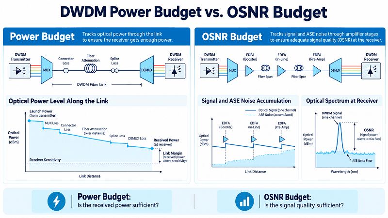
The power budget and OSNR budget answer different questions.

Item	Power budget	OSNR budget
Question	Does enough optical power reach the receiver?	Is signal quality sufficient for the selected format?
Inputs	Transmit power, path loss, receiver sensitivity and limits, design margin	Per-channel power, amplifier noise figure and gain, span loss/count, and relevant impairments
Output	Received power and link margin	Estimated OSNR versus required OSNR
Typical failure	Excessive loss or power outside the receiver’s operating range	Accumulated noise or other impairments leave insufficient margin
Possible remedies	Reduce loss, revise spans, or use compatible amplification/optics	Optimize spans and amplifiers, adjust launch power, use a more robust format, or regenerate

A link can pass one budget and fail the other. For coherent systems, OSNR is important, but it may not fully describe nonlinear penalties; a system-specific model may also use GSNR.

Inputs You Need Before You Start

You can’t design against numbers you haven’t collected. Pull these first.

• Route length and span-by-span distances, measured not estimated
• Fiber type and condition, including splice count and legacy sections
• Site power, space, and cooling at every amplifier location
• Target capacity today plus a growth horizon of 3 to 5 years
• Protection requirement, usually an SLA question rather than an engineering one
• Existing channel plan if the route is already lit

If you are new to the multiplexing layer, the DWDM complete guide covers channels and components before budgeting.

DWDM Topology and Wavelength Planning

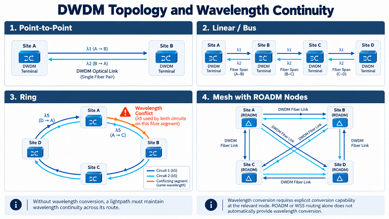
Topology is not just a drawing exercise. It determines which protection schemes are practical and how difficult wavelength assignment may become.

Topology	Protection options	Wavelength reuse	Relative cost	Typical fit
Point-to-point	OLP or line protection, depending on route diversity	Usually straightforward on a dedicated link	Low	DCI, two-site links
Linear / bus	Limited protection or selected-section protection	Limited by route overlap	Low	Spur routes, access
Hub-and-spoke ring	Ring or hub protection, depending on design	Possible on non-overlapping links	Medium	Metro hub-and-spoke
Meshed ring	Ring or path protection	Possible on disjoint links, subject to wavelength continuity	Medium-high	Metro core
Mesh with ROADMs	Optical path protection/restoration	Reuse on non-overlapping links; conversion may be needed	High	Regional, long-haul

Costs are indicative; actual cost depends on fiber availability, node count, protection requirements, and equipment architecture.

The Wavelength Continuity Constraint

An optical circuit generally uses the same wavelength on every segment it crosses unless an intermediate node supports wavelength conversion. Two circuits cannot use the same wavelength on the same fiber segment at the same time, even if their paths do not share a node. Wavelength reuse is possible on links the circuits do not share, subject to continuity and conversion constraints.

Tomás encountered this in an illustrative four-node metro ring carrying 40 wavelengths. His spreadsheet showed channel 21 as free because no individual node appeared to use it twice, but two circuits shared that wavelength on the west-side segment. The records were eighteen months out of date. He caught the conflict during a pre-cutover grid review, preventing an outage. A two-hour review stood between a clean turn-up and a ring that could have dropped half its traffic.

That is why channel planning is a topology problem as well as a spreadsheet task. The DWDM channels guide covers the ITU-T G.694.1 grid, including flex-grid options.

When Wavelength Conversion Pays

A ROADM or WSS can select, route, and add/drop wavelengths, but it does not inherently convert one wavelength to another. Wavelength continuity can be relaxed only when a node supports wavelength-conversion functionality, implemented through OEO conversion or, where supported, an all-optical converter.

OEO conversion adds cost, power consumption, and potential failure points. Use conversion only where it is needed to make the routing and wavelength plan work; converting at every junction can add unnecessary complexity.

The DWDM Power Budget

Does enough optical power arrive at the receiver? First distinguish the available loss budget from the actual link margin.

Available loss budget = transmitter launch power − receiver sensitivity.

Received power = transmitter launch power − total path loss.

Link margin = received power − receiver sensitivity.

Launch power and receiver sensitivity are expressed in dBm; path loss and margin are expressed in dB. Also check the receiver’s maximum input power—a link can have too much power as well as too little.

Path loss includes fiber attenuation, splice and connector loss, mux/demux insertion loss, OADM express loss, and patch-panel loss. On amplified routes, calculate each span and amplifier stage separately; amplifier gain does not remove the route’s physical loss, and its gain, output power, noise, and receiver limits must also be checked.

A Worked Example

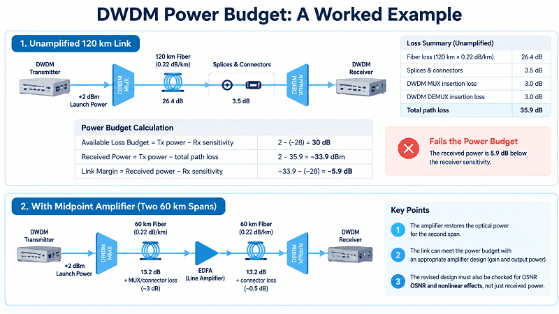
Consider an illustrative 120 km route using G.652.D fiber on a 10G system.

• Fiber: 120 km × 0.22 dB/km = 26.4 dB
• Splices and connectors: 3.5 dB
• Mux and demux insertion loss: 6 dB total across both ends
• Total path loss: 35.9 dB

Assume +2 dBm launch power and −28 dBm receiver sensitivity. The available loss budget is 30 dB, while the path loss is 35.9 dB. Received power would be about −33.9 dBm, leaving a link margin of −5.9 dB before additional design margin.

The link does not close; it is short by about 5.9 dB.

One option is to increase launch power, but transmitter and receiver limits and nonlinear penalties constrain that approach. Another is to split the route into two 60 km spans with a midpoint amplifier. Under these assumptions, each half has roughly 18 dB of loss, including its share of fiber, connections, and terminal mux or demux loss. An appropriately specified amplifier can restore the signal level before the second span.

This may solve the power-budget problem, but amplifier gain and output power must be checked, and OSNR and nonlinear penalties must be recalculated.

Don’t Skip the Margins

A design with only 0.5 dB of headroom may be too fragile. Margins should reflect project requirements and uncertainty, not arbitrary fixed values.

As an illustrative allowance, a design might reserve around 3 dB of system margin and another 1 to 2 dB for a defined repair scenario. These are not universal requirements. Consider repair splices, connector changes, temperature-related variation where relevant, and measurement uncertainty, while avoiding double-counting allowances already included in specifications.

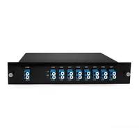
Mux and demux insertion loss should come from the actual datasheet. Specified low-loss components can preserve margin in a tight design. See the DWDM mux and demux guide and FiberMall’s low-insertion-loss DWDM MUX/DEMUX product.

The DWDM OSNR Budget

Noise from optical amplifiers accumulates along an amplified route. The OSNR budget estimates whether signal quality at the receiver is sufficient for the selected modulation format and performance target.

For a simplified chain of similar amplified spans, a useful first-pass estimate is:

OSNR (dB) ≈ 58 + P_ch,in − NF − 10·log10(N)

where P_ch,in is the per-channel signal power at the amplifier input in dBm, NF is the amplifier noise figure in dB, and N is the number of comparable amplifier stages contributing noise. The constant 58 is an approximate reference-bandwidth conversion for a 0.1 nm OSNR measurement near 1550 nm.

If using amplifier output power instead, the equivalent form is:

OSNR (dB) ≈ 58 + P_ch,out − NF − G − 10·log10(N)

Here P_ch,out is per-channel output power in dBm and G is amplifier gain in dB. Use one form consistently; do not combine input power with the output-power formula.

This heuristic assumes comparable spans and amplifiers. Mixed span lengths, Raman amplification, ROADM cascades, channel-dependent gain, and significant nonlinear effects require a span-by-span model. Use the estimate for initial screening, not as a final purchasing decision.

A Worked Example at 96 Channels

Consider a four-span route with 100 km per span, G.652.D fiber at 0.21 dB/km, 1.5 dB of splice/connector loss, and amplifiers with 22.5 dB gain and a 5.5 dB noise figure. Each span has about 22.5 dB loss.

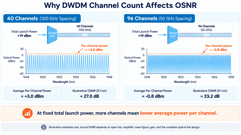
At 96 channels and +19 dBm aggregate WDM launch power, average per-channel power is:

19 − 10·log10(96) ≈ −0.8 dBm.

After 22.5 dB span loss, per-channel power at the next amplifier input is about −23.3 dBm.

Using the simplified input-power formula:

58 − 23.3 − 5.5 − 10·log10(4) ≈ 23.2 dB.

For illustration, assume a particular 400G DP-16QAM implementation requires about 21 dB OSNR under its specified baud rate, FEC, and measurement conditions. That leaves about 2 dB of estimated margin. If a particular 800G implementation requires about 27 dB under its own specifications, the route would not meet that target without a design change. These are examples, not universal thresholds; confirm the actual requirements in the transceiver and line-system specifications and use a consistent OSNR reference bandwidth.

Why Channel Count Costs You OSNR

If the same route carries 40 channels at the same aggregate launch power, average per-channel power rises to:

19 − 10·log10(40) ≈ +3.0 dBm.

Under the same simplified assumptions, estimated OSNR rises to about 27.0 dB. The difference is about 3.8 dB, matching 10·log10(96/40). At fixed aggregate launch power, each doubling of channel count reduces average per-channel power and, in this simplified model, reduces estimated OSNR by about 3 dB.

Increasing aggregate launch power to recover the difference is not always safe. In some G.652.D systems, aggregate launch powers in the high-teens to low-20s dBm may approach the optimum operating point or a nonlinear limit. The +17 to +21 dBm range is not a universal ceiling: the optimum depends on span design, fiber properties, channel spacing and count, baud rate, modulation, and amplifier configuration. Beyond the optimum, more power can increase nonlinear penalties rather than improve performance.

That was the problem in Priya’s illustrative scenario. Her team’s 40-channel link at +19 dBm had an estimated OSNR near 27 dB. At 96 channels, the same aggregate power reduced it to about 23.2 dB. Channel-power imbalance, spectral tilt, and nonlinear interactions further reduced margin on some mid-band channels. Power equalization and spectrum flattening recovered much of the margin, but their effectiveness must be verified with measurements and a system-specific model that considers relevant effects such as SPM, XPM, FWM, or GSNR.

Capacity upgrades can destabilize previously working links. Re-run power, OSNR, and nonlinear assessments whenever channel count, grid, baud rate, or modulation format changes.

Why Span Count Hurts More Than Span Length

In the simplified equation above, doubling the number of otherwise comparable amplifier stages adds about 3 dB to the accumulated-noise penalty. Real spans are not always comparable, however.

Eight 40 km spans and four 80 km spans over the same 320 km route have different span losses and require different amplifier gains. The route with more amplifiers is not automatically worse by exactly 3 dB; gain, noise figure, span loss, and nonlinear behavior all affect the result.

Compare candidate layouts with a span-by-span model. Fewer, longer spans may reduce amplifier-site requirements, but only where the power budget, OSNR, nonlinear performance, equipment, and site constraints allow it. That is the trade-off between the two budgets.

For amplifier gain, noise figure, and Raman options, see EDFA in DWDM. For OSNR requirements by modulation format and the relationship between channel width and baud rate, see the coherent DWDM guide.

Span Design and Regeneration

Amplifier Spacing

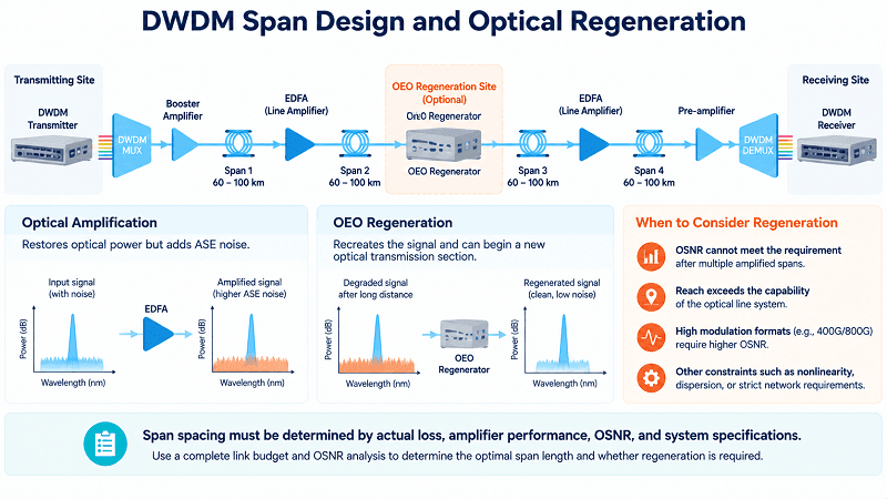
Eighty kilometers is the practical default for G.652.D. About 100 km works with low-loss fiber and careful design. Span loss, not distance, is the real constraint: target 20 to 24 dB per span.

Most links want a booster at the transmit end, line amplifiers between, and a pre-amp at the receive end. The pre-amp matters more than people expect, because noise figure at the receiver sits directly in the OSNR equation.

Dispersion and PMD

Coherent DSP compensates chromatic dispersion and polarization mode dispersion electrically, so dispersion maps are largely a legacy direct-detect concern now. Accumulated dispersion still has to fall inside the module’s compensation range, though. Check the number.

Fiber choice matters. G.653 has zero dispersion near 1550 nm, exactly where four-wave mixing hurts most, so it’s a poor DWDM choice. G.652.D or G.655 are the usual answers. G.654.E raises the nonlinearity threshold and shows up on long-haul builds for that reason.

When to Regenerate

Regenerate when OSNR falls below what the format requires, or when accumulated dispersion exceeds the DSP range. Either condition is a hard stop.

The comparison is rarely regeneration against nothing. It’s regeneration against dropping to a lower-order modulation or a lower rate on that path. A 400G channel that needs a regeneration site might close as 200G without one, and the regenerator costs a transponder pair plus a shelf plus power.

Put regeneration sites where you already have a hut, power, and space. Building a new site for one regenerator is how projects double in cost.

Span design is where DWDM network design stops being a spreadsheet and starts being a site survey. The amplifier locations you can actually get power to constrain everything else.

Protection Design

What happens when a fiber breaks is a design decision. Leaving it to default behavior may not meet the service requirement.

Scheme	Layer	Typical protection target	Indicative switching time	Relative cost
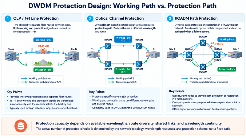
OLP (1+1 or 1:1)	Optical line / fiber path	Line failure, if the protection route is sufficiently diverse	Milliseconds to tens of milliseconds, implementation-dependent	Low-medium
OMSP	Optical multiplex section	Failure affecting the protected section; exact coverage depends on scheme	Often tens of milliseconds; verify platform	Medium
OChP	Optical channel	Failure affecting an individual wavelength	Platform-dependent, often tens of milliseconds	Medium-high
ROADM path protection	Optical path	Working-path failure when a viable diverse backup path exists	Tens to hundreds of milliseconds in some implementations	High

Switching times are indicative only. Actual behavior depends on equipment, architecture, fault type, route diversity, and configuration.

Choosing a Scheme

For a two-site link, OLP can be economical, but it protects against a cable cut only if the protection route is physically diverse enough. Two fibers in the same cable or duct can both be cut by the same excavation.

For a ring with a hub, consider an optical-layer ring or hub protection scheme supported by the topology and equipment. For a ROADM-based mesh, path protection or restoration may be appropriate if an alternate path and sufficient wavelength resources are available.

Dual-homing at the IP layer can protect against some router or interface failures, but it does not protect traffic if redundant links share the same vulnerable conduit.

In DWDM network design, protection must be considered during path and wavelength planning, not only when hardware is selected.

The Wavelength Cost of Protection

A 1+1 scheme typically reserves wavelength capacity on both the working and protection paths. Path protection also consumes resources along the backup path. The capacity impact depends on whether paths use separate fibers, share links, or compete for a common wavelength pool.

Plan for protected capacity, not just working traffic. A 40-channel system may support only 20 protected circuits if every circuit must reserve two channels from the same constrained 40-channel resource pool. If working and protection paths have separate, independently available 40-channel resources, the result can differ. Model the actual routes and wavelength constraints rather than applying a blanket divide-by-two rule.

For ring add/drop configuration and express loss at intermediate nodes, see the DWDM OADM guide.

Commissioning a DWDM Network Design

The design is a hypothesis until you measure it. Acceptance testing is where you find out whether the arithmetic was right, and it’s the step most often compressed when a project runs late. Work through these in order:

1. Measure per-channel launch power and total power into the first span

2. Measure span loss on every span against the design value

3. Measure OSNR at each receive point against the predicted value

4. Read pre-FEC BER per channel and confirm margin above the FEC threshold

5. Sweep the spectrum with an OSA for channel presence, power, tilt, and flatness

6. Verify passband at every ROADM and OADM drop point

7. Cut the working path, measure switch time, confirm traffic restores

8. Record the as-built channel plan, power levels, and modulation assignment

If measured OSNR is 3 dB below prediction, possible causes include unexpected span loss, amplifier gain or noise-figure differences, channel-power imbalance, filtering, or mismatched measurement settings. A poor splice may contribute to excess loss, but the cause should be isolated through measurements rather than assumed.

The as-built document should include assigned wavelengths, measured per-span loss, per-channel power and OSNR at relevant nodes, the protection scheme and measured switching times, and the assumptions behind the original budget.

The Fiber Optic Association’s design methodology is a useful cross-check for the loss-budget side. Cisco’s DWDM planning guide provides more background on optical link modeling.

FAQ

What are the key steps in DWDM network design?

Collect route and fiber data, choose a topology, calculate the power budget and OSNR, design spans and regeneration, plan protection, then commission the system and record as-built values.

How do you calculate a DWDM link budget?

Calculate the available loss budget by subtracting receiver sensitivity from transmitter launch power. Calculate received power by subtracting path loss from launch power, then compare it with receiver sensitivity to determine link margin. Path loss includes fiber attenuation, splices, connectors, mux/demux loss, and OADM express loss.

What’s the difference between a power budget and an OSNR budget?

The power budget asks whether enough optical power reaches the receiver. The OSNR budget asks whether signal quality is sufficient for the selected format. A link can pass one check and fail the other.

How many spans can a DWDM link have before regeneration is needed?

It depends on OSNR or GSNR, span loss, amplifier noise figure, modulation format, and other system constraints—not on a fixed distance or count. Some long-haul coherent systems use 20 or more amplified spans, while some 800G metro designs may need regeneration after only a few. These are examples, not universal rules.

What is the wavelength continuity constraint?

An optical circuit generally must use the same wavelength on every segment unless a node supports wavelength conversion. Two circuits cannot use the same wavelength on the same fiber segment at the same time, even if their paths do not share a node.

Conclusion

DWDM network design comes down to a few rules that are easy to state and easy to overlook.

The power budget and OSNR budget are different calculations. Run both, and use a system-specific model when the route or performance target requires more detail.

Topology and protection choices constrain available paths before hardware is selected, while wavelength continuity makes channel planning a routing problem as well as a spreadsheet task. At fixed aggregate launch power, adding channels reduces per-channel power and can reduce OSNR margin. That is one reason capacity upgrades can destabilize links that previously worked well.

The design is not proven until it has been measured during commissioning.

Priya’s team got its 96 channels running in the end with power equalization, a flatter spectrum, and one regeneration site that had not been planned. The next upgrade on that route went through a nonlinear and span-by-span assessment first.

Send FiberMall your route, span lengths, fiber type, and target capacity, and our optical transport engineers can review the design against the relevant module and line-system specifications before you commit.