ROADM Architecture: Degrees, CDC, and WSS Explained

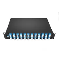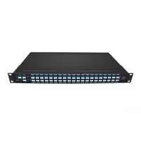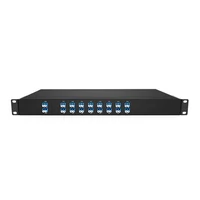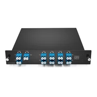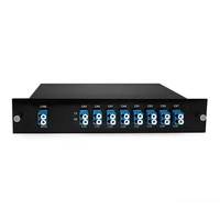
A 20-degree ROADM site can consume three equipment cabinets, more than a hundred circuit boards, and around 400 fibers inside the building. The wavelengths move in software. The hardware does not. In one engineering example documented by ZTE, a node of this scale requires substantial cabinet space, board capacity, and internal fiber management.

That gap is where ROADM projects go wrong. Teams sometimes size a node mainly by channel count, even though channel count alone does not describe the switching architecture or the physical resources required. Degree count, add/drop capacity, CDC capability, and the chosen node architecture all affect hardware, floor space, and power consumption.

This guide works through a ROADM from the inside out: what the switching element actually does, why degree count affects the rest of the design, what each step up the CDC ladder adds, and how to specify a node without overspending. If you already have a topology and a wavelength plan, send both to FiberMall’s optical engineers, and we’ll help size the equipment around the node.

What Is a ROADM?

A reconfigurable optical add-drop multiplexer (ROADM) is a DWDM node that allows individual wavelengths to be added, dropped, or passed through the network under remote control. The level of flexibility depends on the node architecture. Some designs provide limited or wavelength-specific add/drop functions, while colorless, directionless, and contentionless (CDC) designs offer more flexible wavelength and direction assignment.

Many modern WSS-based ROADMs use wavelength selective switches to route optical channels. By contrast, a fixed OADM typically uses passive filters designed for specific wavelengths. If the wavelength plan changes, the fixed OADM may require physical repatching or a module replacement. A suitably configured ROADM can reassign supported wavelengths remotely through its network management system.

“Reconfigurable” sounds like a feature. It is really a trade. You pay for switching hardware, insertion loss, rack units, and power, and what you buy is the ability to change wavelength routing without sending a technician to a remote site for every adjustment. That trade is worthwhile at some sites and not at others, and the rest of this article explains how to tell the difference.

The WSS: What Makes a ROADM Reconfigurable

The wavelength selective switch (WSS) is a key switching element in many modern ROADM architectures. Other components, including amplifiers, optical monitors, and patch panels, support the switching function and help maintain the required optical performance.

How a Wavelength Selective Switch Works

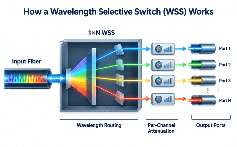
A typical 1×N WSS accepts an input optical signal, separates its wavelength channels internally, and routes each channel to a selected output port. It provides independent per-wavelength routing, allowing different channels to follow different paths through the node. Other WSS configurations, including different input and output port counts, are also available.

Two capabilities matter beyond the port count. The first is per-channel attenuation. Many WSS products can adjust the power of individual wavelength channels, making the device useful for both wavelength routing and optical power equalization. The exact attenuation range and control features depend on the product.

The second is how the WSS is used in the node’s line-side architecture. A bidirectional line normally carries traffic in both directions, and a ROADM must handle the corresponding transmit and receive paths. Multi-degree designs therefore use optical switching resources for the relevant line directions, but the number and arrangement of WSS devices depend on whether the node uses broadcast-and-select, route-and-select, or another architecture.

That is why degree count affects hardware. Each additional line direction generally adds switching interfaces and may add amplification and monitoring requirements. The precise WSS count and equipment layout depend on the vendor’s implementation and the node design.

MEMS vs LC vs LCoS

Several switching technologies are used in WSS designs. The choice affects spectral flexibility, port configuration, optical performance, control complexity, and cost.

Technology	Grid support	Port count	Maturity	Watch out
MEMS	Commonly used in fixed-grid systems; flex-grid support depends on the product design	Moderate to high in many products	Mature, widely deployed	Check the specific product’s channel-width and flex-grid specifications
LCoS	Widely used for flexible-grid WSS, with fine-grained spectral control	Product-dependent; high-port-count designs are available	Established in commercial optical systems	Higher system and control complexity may affect cost
Silicon photonics	Capabilities depend on the specific switching design	Product-dependent	Developing, with a smaller ROADM WSS ecosystem	Verify commercial availability, port count, and system-level performance

LCoS (liquid crystal on silicon) is itself a liquid-crystal-based technology, so it should not be presented as a category mutually exclusive of LC. It is listed separately here because it is a distinct and widely used WSS implementation.

LCoS WSS technology is widely used in flexible-grid applications because it can provide fine-grained control of the optical spectrum. That matters if you plan to carry superchannels or channels with non-uniform spectral widths, which are supported by the flex-grid framework in ITU-T G.694.1 and must be reflected in the DWDM channel plan.

MEMS WSS products have traditionally been widely deployed in fixed-grid systems, but it is too broad to say that MEMS technology can never support flexible-grid operation. Flex-grid support depends on the specific WSS design and its spectral resolution and control capabilities. When comparing products, check the supported grid, slot-width range, channel spacing, and spectral performance rather than assuming capability from the switching technology alone.

Degrees: The Number That Sets Everything Else

When estimating ROADM cost and complexity, degree count is one of the first things to establish. Channel count matters too, but it does not describe how many line directions the node must connect or how much switching hardware those connections require.

What a Degree Is

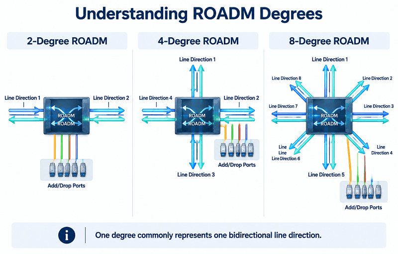
A ROADM degree is one line-side direction connecting the node to another network node. In a conventional bidirectional system, a degree commonly corresponds to a pair of fibers, one for each direction of transmission.

A 2-degree ROADM connects two line-side directions, as commonly found on a linear route or at a node in a ring. It can pass wavelengths between those directions while adding or dropping selected channels locally. It is not simply an inline amplifier: its switching and add/drop functions depend on the ROADM architecture.

At 3 degrees and above, the node can connect to more neighboring directions and may serve as a network junction. Depending on its internal switching architecture, wavelengths can be routed between supported line directions. An 8-degree node has eight line-side directions, but the degree count alone does not guarantee that every wavelength can be routed freely between every pair of directions; that depends on the node’s switching design and configuration.

What Each Added Degree Costs

This is the part that surprises people. Adding a degree is not simply adding a port. It adds another line-side connection and usually increases the switching, amplification, monitoring, and cabling resources required by the node.

Degree count	Typical role	What it adds	Site impact
2	Linear or ring node	Switching resources for two line directions; add/drop hardware depends on the design	Often a relatively compact installation
3–4	Small junction	Additional line-side switching interfaces and potentially more amplification and monitoring	More equipment and fiber management than a two-degree node
8	Metro core node	A larger WSS or optical switching set, OCM, and more patching interfaces as required	Higher cabling density; rack needs depend on platform integration
16–20	Regional hub	Extensive line-side switching, add/drop capacity, and dense fiber interconnection	May require multiple racks or cabinets, depending on the system

ZTE’s engineering write-up on optical cross-connects provides a concrete example of the physical scale involved: its 20-degree ROADM example can require three cabinets, more than 100 boards, and roughly 400 fibers terminating inside the station. This illustrates the optical cross-connect reality behind a node that looks tidy on a topology diagram. These figures describe that particular implementation, not a universal requirement for every 20-degree ROADM.

Marta found this the expensive way. She scoped a metro junction at 4 degrees in 2021, with growth to 6. By 2024, the site was running 11 degrees after two acquisitions added fiber routes.

The wavelengths were fine. The rack was not. She spent a quarter negotiating space in a building that had none, and the eventual answer was to split the node across two rooms with a fiber run between them.

Plan degree count for the topology you expect in five years, not just the one on today’s drawing. It is one of the hardest design dimensions to change later because adding line directions can require new switching hardware, cabling, space, and power.

Broadcast-and-Select vs Route-and-Select

Two common multi-degree ROADM architectures perform wavelength routing in different ways, with different hardware requirements and optical-loss characteristics.

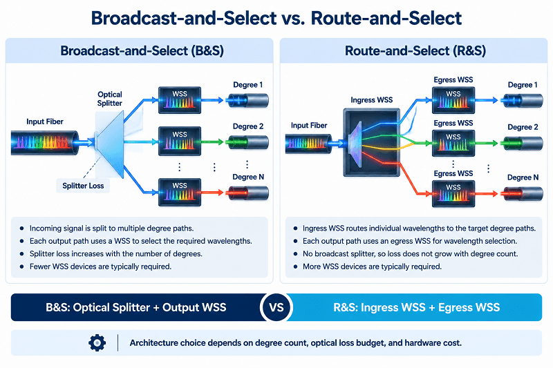
Broadcast-and-select splits an incoming signal so that it is distributed to multiple degree paths. A WSS on each relevant output path then selects the wavelengths that should continue in that direction. This architecture can require fewer WSS devices than route-and-select, depending on the design. Its main trade-off is splitter loss: the optical power is divided among the output paths, and the resulting loss must be included in the link budget.

Route-and-select uses WSS switching at the input and output stages to route wavelengths between line directions rather than broadcasting the incoming signal to all directions and filtering it at the outputs. It generally avoids the degree-dependent splitter loss associated with broadcast-and-select, but it requires more WSS resources and can increase hardware cost and complexity.

At lower degree counts, broadcast-and-select may be a cost-effective choice if the optical loss budget allows it. As degree count increases, splitter loss can make route-and-select more attractive. There is no universal eight-degree threshold: the preferred architecture depends on the WSS configuration, optical link budget, required performance, and vendor platform. Ask which architecture a quote assumes, because the two are not interchangeable at the same price.

Why Degrees Enable Restoration

A 2-degree node connects two line-side directions. That does not mean the wider network has only one possible path. For example, a two-degree node in a ring may still participate in an alternative route through the other nodes in the ring.

A node with three or more degrees provides additional line-side directions, which can create more routing options. However, the existence of an alternative direction at one node does not by itself guarantee end-to-end restoration. Restoration depends on the network topology, available wavelengths or spectrum, internal switching capabilities, and the control and protection mechanisms deployed across the network.

That is the real argument for degree count: additional degrees can provide the physical routing options needed for optical-layer protection or restoration, provided the wider network has a viable alternate path and sufficient resources.

Two mechanisms do the work. Optical protection pre-establishes a backup path and switches traffic when the working path fails. Some protection schemes are designed for switching times around tens of milliseconds, but actual performance depends on the protection method and equipment. Optical restoration establishes or computes a new route after a failure. It is generally slower than pre-planned protection, but it can use shared spare capacity more efficiently, depending on the restoration scheme and network design.

Wavelength Switched Optical Networks (WSONs) can use control-plane frameworks such as GMPLS and PCE to support routing and wavelength assignment. These frameworks are described in IETF RFC 6163. They are not the only way to automate ROADM reconfiguration: deployments may also use SDN controllers, network management systems, or vendor-specific control systems. Without an automated control plane, operators may still reconfigure the node remotely through the management system, although network-wide restoration may require additional coordination or manual intervention.

This is also where contentionless capability can help. A node that has internal wavelength contention may block an add/drop or restoration request even when line-side capacity is available. Contentionless switching can reduce this type of internal blocking, but it does not by itself guarantee end-to-end restoration; the network still needs a valid route and available resources.

Colorless, Directionless, Contentionless: The CDC Ladder

 The DWDM complete guide defines these terms. What matters for a purchase is what each capability allows the network to do and what additional hardware or switching resources the chosen implementation requires.

What Each Step Adds in Hardware

Each rung of the ladder adds a specific capability. The components used to implement it vary by vendor and architecture.

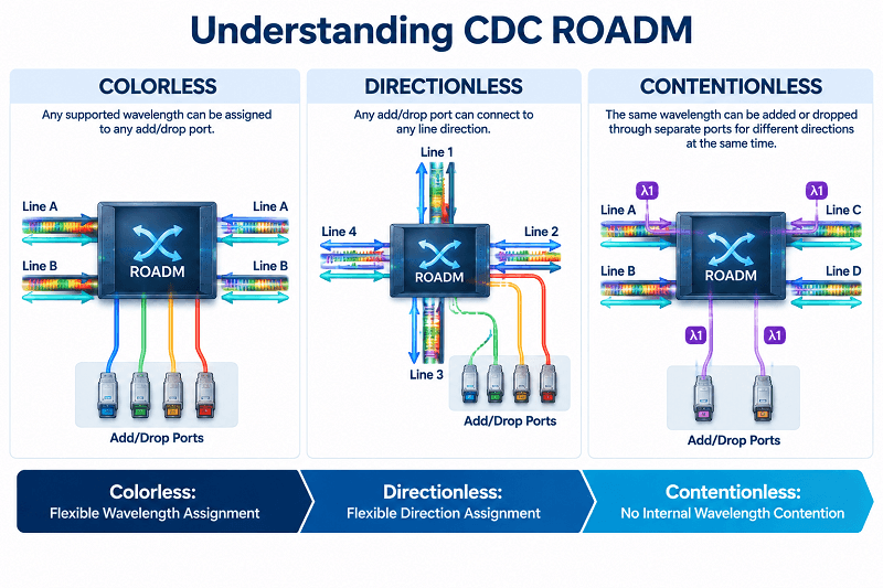
Colorless means that any supported wavelength can be assigned to any add/drop port, rather than each port being permanently tied to a particular wavelength. Colorless functionality can be implemented through wavelength-selective add/drop switching and compatible transponders, often including tunable transponders. The exact hardware arrangement varies by platform.

Directionless means that an add/drop port can be connected to any supported line direction. Implementations may use optical multicast switches (MCSs), WSS devices, or other switching elements to connect add/drop signals to the required degree.

Contentionless means that the same wavelength can be added or dropped simultaneously through separate add/drop ports for different directions without internal wavelength contention. This capability requires a switching architecture that can handle duplicate-wavelength add/drop requests; implementations may use multicast switches, M×N WSSs, or other optical switching fabrics.

So the ladder is: flexible wavelength assignment, flexible line-direction assignment, and then the ability to handle duplicate wavelengths on separate add/drop paths without internal contention. Each step adds operational freedom and may add hardware or control complexity. Combining all three produces a CDC ROADM, which is often considered for high-capacity hub builds but is not automatically necessary for every new deployment.

What Each Step Buys You

Colorless operation can simplify sparing and wavelength planning. A compatible tunable transponder can be assigned to different supported wavelength slots and add/drop ports, making it easier to share spare units. The spare must still match the required line rate, reach, modulation, and platform compatibility requirements.

Directionless operation decouples add/drop ports from fixed line directions. A transponder can be provisioned toward a supported neighboring direction without manually repatching the optical path, which can simplify maintenance and rerouting.

Contentionless operation reduces internal blocking when multiple circuits using the same wavelength need to be added or dropped through different ports and directions. It can improve routing flexibility, but the available port count and switching capacity still need to be sized for the traffic plan.

Where Most Metro Builds Actually Land

A colorless and directionless (CD) design may be sufficient for many metro rings. Contentionless capability is more likely to justify its additional cost at nodes where many same-wavelength circuits need to converge or where flexible add/drop behavior across several directions is an important restoration requirement. The right choice depends on the traffic matrix and restoration plan, not simply on the size of the network.

Kenji’s team bought contentionless capability for a six-node metro ring. The business case was flexibility. Two years later, no circuit had needed duplicate-wavelength add/drop at the same node, and the multicast switches had consumed budget that could have funded a second route out of the ring.

The capability was real. The need was not.

Buy the CDC level your traffic and restoration plans require. Specifying CDC everywhere without a clear operational need can be an expensive habit in optical transport.

ROADM vs OADM: Choosing the Right Add/Drop

	Fixed OADM	ROADM
Wavelength assignment	Fixed by the filter design	Remotely configurable; flexibility depends on the ROADM architecture
Reconfiguration	Usually requires physical repatching or module changes	Remote reconfiguration for supported functions
Typical deployment	Point-to-point links, spurs, or stable ring applications	Linear, ring, and multi-degree network nodes; degree depends on the platform
Per-channel power control	Not typically provided by the passive OADM itself	Often available through WSS attenuation, depending on the product
Mesh restoration	No dynamic wavelength switching at the OADM node	Can support optical-layer restoration when the node and wider network are designed for it
Cost	Generally lower	Generally higher; varies with degree count, add/drop capacity, CDC level, and vendor
Best fit	Stable wavelength plans and simple add/drop requirements	Changing wavelength plans, multi-direction routing, and restoration requirements

A fixed OADM is the right answer more often than vendors suggest. If the wavelength plan is stable, the ring is simple, and nobody needs dynamic wavelength switching at the node, a passive module can do the job at a fraction of the cost. FiberMall stocks passive OADM modules for exactly those sites, and the DWDM OADM guide covers module selection in detail.

A ROADM earns its price when the wavelength plan changes, when optical-layer protection or restoration is required, or when per-channel power control helps manage the optical link budget. Those are real requirements. “Flexibility” on its own is not one.

What a ROADM Node Still Needs Around It

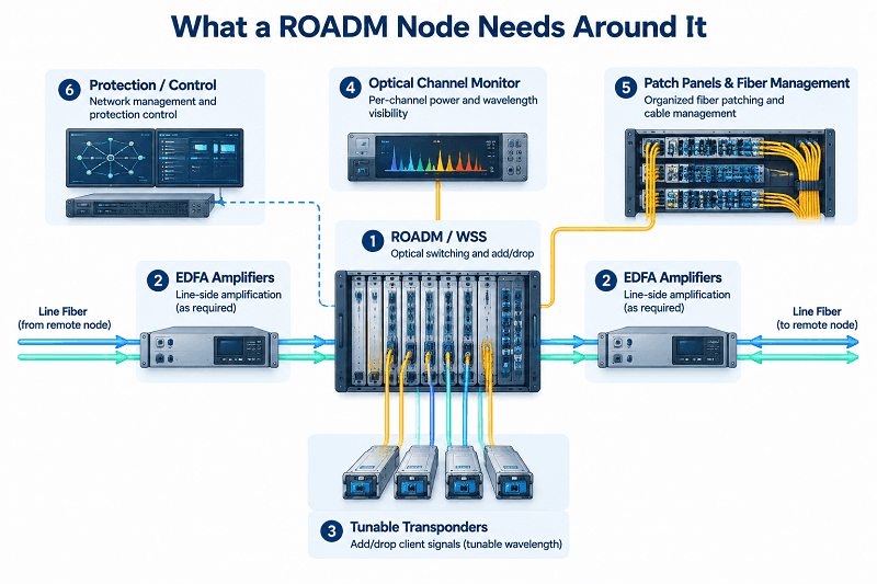
The ROADM line cards are only part of the node. Budget for the supporting equipment and site requirements, or the project may run into unexpected costs.

Amplifiers depend on degree count and the optical link budget. A multi-degree node may need amplification on multiple line directions, as well as amplification on add/drop paths where required. However, amplifier functions may be integrated into optical line boards, and the number and placement of amplifiers depend on span loss, WSS insertion loss, launch-power requirements, and the system architecture. The EDFA amplifier product range provides options for different optical amplification requirements.

Transceivers at a colorless ROADM are often tunable. In a colorless design, tunable transponders can be assigned to different supported wavelengths, simplifying provisioning and potentially reducing the number of wavelength-specific spares. Fixed-wavelength optics may still be appropriate in colored or otherwise wavelength-specific architectures. The coherent DWDM guide covers the OSNR considerations associated with coherent transmission and higher-order modulation formats.

Optical channel monitors provide visibility into per-channel power and wavelength information, helping operators monitor the performance of WSS-based nodes. OSNR monitoring may also be available when the system includes suitable optical performance monitoring functions; it should not be assumed that every OCM provides the same OSNR measurement capability.

Patch panels and fiber management are unglamorous and, at high degree counts, can become major design constraints. A site with hundreds of internal fibers needs careful planning for routing, labeling, access, and future expansion.

Protection switching may be implemented within the line system or through separate equipment, depending on the protection architecture. Some systems support protection functions within their optical transport platform; others may use an external optical line protection switch for specific client or line-side applications. Confirm where protection is implemented, because this affects port requirements, interoperability, and the failure scenarios the design can handle.

Specifying a ROADM

Work in this order. Each step constrains the next.

1. Fix degree count from the five-year topology, not today’s drawing

2. Choose the CDC level from the restoration plan

3. Pick the WSS technology from the grid requirement, fixed or flex

4. Size add/drop ports from the transponder plan

5. Budget amplifiers per degree, not per node

6. Decide the control plane, including whether Open ROADM matters to you

7. Confirm rack space, power, and fiber count at the physical site

8. Verify the management interface against your NMS

Step 6 deserves a note. The Open ROADM MSA publishes disaggregated specifications and YANG models so that line systems and transponders from different vendors can interoperate. If multi-vendor procurement matters to your organization, that compatibility changes the RFP. If you intend to buy a single vendor’s line system end to end, it changes nothing.

FAQ

What does ROADM stand for?

Reconfigurable optical add-drop multiplexer. It is a DWDM node that allows wavelengths to be added, dropped, or passed through the network under remote control. The degree of wavelength and direction flexibility depends on its architecture.

What is the difference between ROADM and OADM?

A fixed OADM uses filters that define which wavelengths can be added or dropped, so changing the wavelength plan usually requires physical changes. A ROADM supports remote reconfiguration of wavelength routing, with the available flexibility depending on its switching and add/drop architecture.

What is a 2-degree vs. 8-degree ROADM?

Degree count is the number of line-side directions connected to a node. In conventional bidirectional systems, each degree commonly corresponds to a fiber pair. A 2-degree node connects two line directions, often on a linear route or ring. An 8-degree node connects eight line directions, with internal routing capabilities determined by its architecture.

What does colorless, directionless, contentionless mean?

Colorless means supported wavelengths can be assigned to any add/drop port. Directionless means add/drop ports can connect to any supported line direction. Contentionless means the same wavelength can be added or dropped through separate ports for different directions without internal wavelength contention. Each capability adds flexibility and may increase hardware or control complexity.

How much does a ROADM node cost?

Cost depends on degree count, add/drop capacity, CDC level, WSS architecture, amplification, monitoring, and the vendor platform. There is no meaningful universal price. Build the estimate around the required switching resources, amplifiers, add/drop components, rack space, power, and fiber management rather than channel count alone.

What is Open ROADM?

Open ROADM is a multi-source agreement that publishes disaggregated ROADM specifications and YANG models to support interoperability between equipment from different vendors. Actual interoperability depends on supported features, specification compliance, and qualification testing.

Conclusion

Selecting a reconfigurable optical add-drop multiplexer comes down to a few rules that are easy to state and expensive to learn on site.

Degree count is a major driver of switching hardware, floor space, and fiber requirements, and it can be difficult to change later. Plan for the topology you expect in five years. CDC is a set of capabilities, not a mandatory package: CD may be sufficient for many metro applications, while contentionless switching is valuable where the traffic and restoration plan require it. WSS technology matters for flex-grid support, but the specific product’s spectral capabilities—not the technology label alone—should guide the decision.

A ROADM node is also more than its line cards. Amplification must be designed around each line direction and the optical link budget; tunable transponders can simplify colorless operation; and optical monitoring helps make reconfiguration manageable.

Ravi learned the amplification point on a 9-degree regional node. He had budgeted one amplifier per site, following the pattern from his 2-degree builds. The bill of materials came back with amplification requirements across multiple directions, and the project had to return for funding before it could move forward.

Send FiberMall your topology, degree count, and wavelength plan, and our engineers will help scope the transceivers, amplifiers, and passive add/drop modules around the node.